Fundamental Concepts of R Language

 Variables in R

A variables are nothing but reserved memory locations to store values. This means that when you create a variable you reserve some space in memory.

Data Operators

1. Arithmetic Operators
2. Assignment Operators
3. Relational Operators
4. Logical Operators
5. Special Operators

1. Arithmetic Operator

    (" + ") → Add two operands or unary plus.
                             >> 2+3
                              5
                              >>+2
    (" - ") → Subtract two operands or unary subtract.
                             >> 3-1
                              2
                              >>-2
    (" * ") → Multiply two operands
                             >> 2*3
                              6
    (" / ") → Divide left operand with the right and results is in float.
                               >> 6/3
                              2.0
    (" ^ ") → Left operand raised to the power of right
                               >> 2^3
                               8
    (" %% ") → Remainder of the division of left operand by the right
                               >>5%%2
                               1
     (" %/% ") →Division that results into whole number adjusted to the left in the number line.
                              >> 7%/%3
                              2
                            
2. Assignment Operators

     (" = ") →  x = <right operand>
                  >>x=5
                  >>x
                   5
     (" <- ") → x <- <right operand>
                    >>5<-15
                     >> x
                      15
     (" <<- ") → x<<-  <right operand>
                       >> x<<-2
                        >> x
                         2
     (" -> ") → <left operand> -> x
                    >> 25 -> x
                      >> x
                       25

3. Relational Operators
     
      (" > ") → True if left operand is greater than the right
                              >> 2>3
                                  False
       (" < ") → True if left operand is less than the right
                               >> 2>3
                                    True
       (" == ") → True if left operand is equal to right
                               >> 2==2
                                     True
        (" != ") → True if left operand is not equal to the right
                                 >> x >>=2
                                  >> print(x)
                                   1
        (" >= ") → True if left operand is greater than or equal to the right operand
                                  >> 2 >=3
                                    False
        (" =< ") → True if left operand is less than or equal to the right operand
                                  >> 2 =<3
                                    True

4. Logical Operators

         (" & ") → Returns x if x is False , y otherwise
                                  >> 2 &3
                                    3
         (" | ") → Returns y if x is False, x otherwise
                                   >> 2|3
                                    2
         (" ! ") → Returns True if x is True, False otherwise
                                   >> !1
                                    False

5. Special Operators
       
         (" : ") → It creates the series of numbers in sequence for a vector
                                      >> x <- 2:8
                                       >> x
                                       [1] 2 3 4 5 6 7 8
         (" %in% ") → This operator is used to identify if an element belongs to a vector
                                        >> x <-2:8
                                        >> y <- 5
                                        >>y %in% x
                                         True

Data Type
 We do not need to declare a variables before using them.
    

Vectors :-
   A Vector is a sequence of data elements of data elements of the same basic type.
      Example :
                 vtr = (1,3,5,7,9)
                  or
                  vtr <- (1,3,5,7,9)
  There are 5 Atomic vectors, also termed as five classes of vectors.

Lists :-

  Lists are the R objects which contain elements of different types like -numbers, strings, vectors and another list inside it.
    > n = c(2,3,5)
    > 5 = c("aa", "bb", "cc", "dd", "ee")
    >x = list(n, s, TRUE)

Arrays :-

Arrays are the R data objects which can store data in more than two dimensions.
It takes vectors as input and uses the values in the dim parameter to create an array.
       vector 1 <- c(5,9,3)
        vector2 <- c(10,11,12,13,14,15)
  result <- array(c(vector1, vector2), dim = c(3,3,2))

Matrices :-

 Matrices are the R objects in which the elements are arranged in a two-dimensional rectangular layout.
A Matrix is created using the matrix() function.
  matrix(data, nrow, ncol, byrow, dimnames)

- data is the input vector which becomes the data elements of the matrix.
- nrow is the number of rows to be created
- ncol is the number of columns to be created.
- byrow is a logical clue. If TRUE then the vector elements are arranged by row.
- dimname is the names assigned to rows and columns.

Factors:-

Factors are the data objects which are used to categorize the data and store it as levels
They can store both strings and integers.
They are useful in data analysis for statistical modeling.

   data <- c("East","West","East","North","North","East","West","West","East")
                   factor_data <- factor(data)

Data Frames :-

  A data frame is a table or two-dimensional array-like structure in which each column contains values of one variable and each row contains one set of values from each column.
   emp_id = c(1:5),
emp_name = c("Rick","Dan","Michelle","Ryan","Gary"),
salary = c(623.3,515.2,611.0,729.0,843.25),
 emp.data <- data.frame(emp_id, emp_name, salary)

Flow Control Statements

if → It evaluates a single condition
if .. else → It evaluates a group of condition and selects the statements
Switch → It checks the different known possibilities and selects the statements 

Loops :-

Repeat → Repeat things until the loop condition is true
While → Repeat things until the loop condition is true
For → Repeat things till the given number of times.

Read More

Introduction of R Language

Why do we need Analytics ?

→ Data analytics helps organizations harness their data and use it to identify few opportunities.
- Cost reduction
- Better marketing & product analysis
- Organization analysis
- Faster, better decision marketing

What is Business Analytics ?

→ Business Analytics examines large and different types of data to uncover hidden patterns, correlations and other insights.

What is Data Visualizations ?

→ Visualization allows us visual access to huge amounts of data in easily digestible visuals.


→ Well designed data graphics are usually the simplest and at the same time, the most powerful.

Why R ?

→ Programming and Statistical Language
⇒ Apart from used as a statistical language, it can also be used a programming language for analytical purposes.

→ Data Analysis and Visualization
⇒ Apart from being one of the most dominant analytics tools, R also is one of the most popular tools used for data visualization.



 
→ Simplest and Easy to Learn
⇒ R is a simple and easy to learn, read and write.





→ Free and Open Source
⇒ R is an example of a FLOSS (Free/Libre and Open Source Software) which means one can freely distribute copies of this software, read it's source code, modify it, etc.

Read More

Java - The Complete Reference by Herbert Schildt

JAVA BOOK

This book is a comprehensive guide to the Java language, describing its syntax, keywords and fundamental programming principles. Significant portions of the Java API library are also examined. This book is for all programmers, whether you are a novice or an experienced pro. The beginner will find its carefully paced discussions and many examples especially helpful.

Download:

Read More

JOINs

The JOIN is used to combine rows from two or more tables.

SQL Inner Join :-

Select all rows from tables for the match between the columns in tables.
Same as JOIN

Syntax :-
SELECT column FROM table1
INNER JOIN table2
on table1.column = table2.column;

[only matching rows are retrieved]

 Example :-

SELECT emp.eno, emp.ename, dept.dno, dept.dname FROM emp
INNER JOIN dept
on emp.dno = dept.dno; 

SQL LEFT JOIN :-

Returns all rows from the left table, with the matching rows in the right table.
The result is NULL in the right side when there is no match.

Syntax :-

SELECT Columns FROM table1
LEFT [OUTER] JOIN table2
on table1.column = table2.column;
 
Example :-
SELECT emp.eno, emp.ename,dept.dno, dept.dname FROM emp
LEFT JOIN dept
on emp dno = dept.dno; 

SQL RIGHT JOIN :-

Returns all rows from the right table, with the matching rows in the left table.
The result is NULL in the left side when there is no match.

Syntax :-

SELECT columns FROM table1
RIGHT [OUTER] JOIN table2
on table1.column = table2.column;

Example :-

 FULL OUTER JOIN

Returns all rows from the left table and from the right table.
The combines the result of both LEFT and RIGHT joins.

Syntax :-

SELECT columns FROM table1
FULL [OUTER] JOIN table2
on table1.column = table2.column;

Example :-

Read More

UNION Operator

Combines the result of two or more select statement.

Each Select Statement must have same number of columns and columns must have same data types.

Columns should also be in same order.

Syntax :-

[ Removes the duplicate Values ]

SELECT Column1, Column2, FROM table1 
UNION 
SELECT Column1, Column2, FROM table2 

[ Duplicate Values are retained ]

SELECT Column FROM table1
UNION ALL
SELECT Column FROM table2


Example :-

SELECT ename, job FROM emp1
UNION
SELECT ename, job FROM emp2

We have two tables :-

After use UNION  operator we get this table,

a

Read More

FOREIGN KEY

A FOREIGN KEY in one table points to PRIMARY KEY in another table.

A foreign key can have a different name than the primary key it comes from.

The primary key used by a foreign key is also known as a parent key. The table where the primary key is from is known as a parent table.

The foreign key can be used to make sure that the row in one table have corresponding row in another table.

Foreign key value can be null, even though primary key value can't.

Foreign key don't have to be unique in fact, they often aren't.

Create table from use a FOREIGN KEY:-

CREATE TABLE department
(
D_id int NOT NULL AUTO_INCREMENT PRIMARY KEY,
D_Name varchar (40),
E_id int,'
CONSTRAINT employee_Eid_fk
FOREIGN KEY (E_id) REFERENCES employee (E_id)

The CONSTRAINT clause allows to define constraints name for the foreign key constraint. If we omit it MySQL will generate a name automatically. It is optional.

The REFERENCES clause specifies the parent table and its columns to which the columns in the child table refer. The number of columns in the child table and parent table specified in the FOREIGN KEY and REFERENCES must be the same.

Read More

ALTER TABLE

This command is used to Add/Change/Modify/Drop existing structure of the table.

ADD Column
Enable/Disable Constraints
Change Column
Modify Column
Drop Column

ADD Column :- When a new column is to be added to the table structure without constraints.

Syntax :-

ALTER TABLE table_name
ADD COLUMN column_name datatype (size);

Example:-

ALTER TABLE my_tab
ADD COLUMN stu_id integer (5);

Change Column :-This is used to change name and data type of an existing column without constraints.

Syntax:-

ALTER TABLE table_name
CHANGE COLUMN old_column_name new_column_name new_data_type (size);

Example:-

ALTER TABLE my_tab
CHANGE COLUMN name student varchar (5);

Modify Column :- This is used to modify size of the data type or the data type itself of an existing column without changing column name.

Syntax:-

ALTER TABLE table_name
MODIFY COLUMN column_name datatype (size);

Example:-

ALTER TABLE  my_tab
MODIFY COLUMN roll integer (10);

DROP COLUMN :- When a column in a table need to delete

Syntax :- 

ALTER TABLE table_name
DROP COLUMN column_name;

Example:-

ALTER TABLE my_tab
DROP COLUMN roll;

When removing constraints from a column

Syntax:-

ALTER TABLE table_name
DROP constraints_name column_name;

Example:-

ALTER TABLE my_tab
DROP UNIQUE KEY (roll);

Read More

SQL The Complete Reference, 3rd Edition Paperback – 1 Jul 2017 by James Groff (Author), Paul Weinberg (Author), Andy Oppel (Author)

SQL The Complete Reference, 3rd Edition

Get comprehensive coverage of every aspect of SQL from three leading industry experts. Revised with coverage of the latest RDBMS software versions, this one-stop guide explains how to build, populate, and administer high-performance databases and develop robust SQL-based applications. 

SQL: The Complete Reference, Third Edition shows you how to work with SQL commands and statements, set up relational databases, load and modify database objects, perform powerful queries, tune performance, and implement reliable security policies. Learn how to employ DDL statements and APIs, integrate XML and Java scripts, use SQL objects, build web servers, handle remote access, and perform distributed transactions. Techniques for managing in-memory, stream, and embedded databases that run on today's mobile, handheld, and wireless devices are included in this in-depth volume.

• Build SQL-based relational databases and applications
• Create, load, and modify database objects using SQL
• Construct and execute simple, multitable, and summary queries
• Implement security measures with authentication, privileges, roles, and views
• Handle database optimization, backup, recovery, and replication
• Work with stored procedures, functions, extensions, triggers, and objects
• Extend functionality using APIs, dynamic SQL, and embedded SQL
• Explore advanced topics such as DBMS transactions, locking mechanisms, materialized views, and two-phase commit protocol
• Understand the latest market trends and the future of SQL

About the Author

James R. Groff is senior vice president of business strategy at Oracle Corporation. He is a SQL expert whose SQL-oriented software company, TimesTen Performance Software, was acquired by Oracle in 2005.

Paul N. Weinberg is senior vice president of NetWeaver MDM at SAP. He is a SQL expert whose SQL-oriented software company, A2i, Inc., was acquired by SAP in 2004. Weinberg is the bestselling author, with James Groff, of the previous editions of this book.

Read More

Auto Increment

Auto increment is used to  generate an unique, when a new record is inserted into a table.
If use a auto increment than increase by 1. 
In table sequence is increment automatically.
Auto increment ignore null value.

Syntax :-

CREATE TABLE table_name
(
Column_name int NOT NULL AUTO_INCREMENT,
Column_name1 varchar (50) NOT NULL,
Column_name2 varchar (50),
PRIMARY KEY (column_name)
);

Example :-

CREATE TABLE emp
(
Emp_id int NOT NULL AUTO_INCREMENT,
Emp_name varchar (50) NOT NULL,
City varchar (50),
PRIMARY KEY (Emp_id)
);

Insert rule are different 

INSERT INTO emp (emp_name, city)
VALUES
('Subham', 'Delhi'),
('Ankit', 'Mumbai');

INSERT INTO emp (emp_id, emp_name, city)
VALUES
(NULL, 'Subham', 'Delhi'),
(NULL, 'Ankit', 'Mumbai');

INSERT INTO emp (emp_id, emp_name, city)
VALUES
(NULL, 'Subham', 'Delhi'),
(1, 'Ankit', 'Mumbai');

Table:-

Use NULL VALUE

Read More

PRIMARY KEY

The PRIMARY KEY constraints uniquely identifies each record in a database table. Primary keys must contain UNIQUE values. A primary key column cannot contain NULL values. Most a tables should have a primary key, and each table can have only ONE primary key.

Example:-

CREATE TABLE student 
(
Name varchar (30),
Roll integer (5) NOT NULL PRIMARY KEY,
Mobile_no integer (10)
);

CREATE TABLE student 
(
Name varchar (30),
Roll integer (5) NOT NULL,
Mobile_no integer (10),
PRIMARY KEY (Roll)
);

Read More

UNIQUE KEY

The UNIQUE constraint uniquely identifies each record in a database table. There can be many UNIQUE constraints per table. 

A Unique key column can contain NULL values.

Syntax :-

   CREATE TABLE student
   (
    Name varchar (30),
    Roll integer (5),
    Mobile_no integer (10) UNIQUE KEY
    );

Example :-

CREATE TABLE u_tab
(
stu_id int (5) UNIQUE KEY,
name varchar (30),
roll int (5) UNIQUE KEY,
city varchar (40)
);

Insert Table :-

Read More

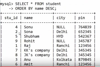
ORDER BY

This is used to sort the record.

ASC - It sorts in ascending order (by default).
DESC - It sorts in descending order.

1. Sorts in descending order

Syntax :-

   SELECT * FROM table_name
   ORDER BY column_name DESC;

Example :-

   SELECT * FROMemp
   ORDER BY emp_name DESC;


 Example :-

Read More

LIKE Operator

The LIKE operator is used to search for a specified pattern in a column.

Syntax :-

    SELECT * FROM table_name
    WHERE column_name LIKE 'pattern';

Example :-

    SELECT * FROM new_tab
    WHERE name LIKE '%nu';

Wildcards:-

Wildcards are used to search for data within a table. These characters are used with the LIKE operator.

1. % - Zero or more characters

    'Irawen%' - All starting with Irawen  Ex:-  Pirawen
    '%shows' - All ending with shows Ex:-  Pirawen
    '%sh%' - All containing with sh.  Ex:-  Pirawen

2.  - One single character

     'show_ '- Starting with show then any character. Ex:-  shows
     '_rawen' - any character then eek.  Ex:- irawen
     'I_r_a' -  I then any character, then r then any character, then a Ex:-  -Irawen

Solve Example :-

Use LIKE operator :-

Read More

BETWEEN Number operator

The BETWEEN operator selects values within a range. The values can be numbers, text, or dates.

1. Between Number

Syntax :- 

  SELECT * FROM table_name
  WHERE column_name BETWEEN value1 and value2;

Example :-

  SELECT * FROM new_tab
  WHERE stu_id BETWEEN 6 and 8;

Solve Example :-

Read More

IN Operator

The IN operator allows you to specify multiple values in a WHERE clause.

Syntax :-

   SELECT * FROM table_name
   WHERE column_name IN ('value1' , 'value2' , ......);

Example :-

  SELECT * FROM table_name
  WHERE name IN ('Anu' , 'Sonu');

New table create 

Solve Example :-

Read More

OR Operator

The OR operator displays a record if either the first condition OR the second condition is true.

Syntax :-

  SELECT * FROM table_name
  WHERE column_name = 'value'
   OR column = 'value';

Example :-

   SELECT * FROM new_tab
   WHERE name = 'Anu'
    OR stu_id = 5;

First we see a table :-
  

Example :-

Read More

AND Operator

The AND operator display a records if both the first condition AND the second condition are true.

Syntax :- 
    SELECT * FROM table_name
    WHERE column_name = 'value'
    AND column = 'value';

Ex:-
 SELECT * FROM new_tab
 WHERE name = 'Anu'
 AND stu_id = '5';

This is a database.

Example :-

Read More

SQL Statements and Rules

SQL command or statement is a special kind of sentence that contains clauses and all end with a semicolon(;) just as a sequence ends with a period.

SQL statements are divided into four sub language:

(i) Data Definition Language (DDL):- It is used to define the structure of tables in the database.It contains the necessary statement to CREATE , RENAME , ALTER and DROP the tables.

(ii) Data Manipulation Language (DML):- It is a used to manipulate the data in the database.It contains statement to UPDATE , DELETE , INSERT and SELECT data that is stored in the database.

(iii)Data Control Language (DCL):- It is used to control data stored in the database.It contains statement give permission to access the data in the database.These statements are GRANT and REVOKE.

(iv) Transaction Control Language(TCL):- It is used to control the transaction in a database system. It contains statements like COMMIT , ROLLBACK and SAVEPOINT.

Rules for SQL Command/Statements

Rules for SQL commands are given below:
* SQL statements are not case sensitive.
* SQL statements can be executed on one or more tables.
* Keywords cannot be abbreviated.
* The statement can be typed in single line or multiple lines.
* Place a semicolon at the end of the SQL statements.
* A comma (,) is used to separate parameters without a clause.
* Characters and data constants or literals must be enclosed in single quotes(' ').

Read More