Python Coding challenge - Day 235 | What is the output of the following Python Code?

 

In Python, memoryview is a built-in class that allows you to access the memory of an object without copying it. This can be useful for performance reasons, especially when dealing with large data sets or when you want to manipulate data in place.

Here's a breakdown of the code snippet you provided:

x = memoryview(b'clcoding')

print(type(x))

Creating a memoryview object:

b'clcoding' is a bytes object. The b prefix indicates that this is a bytes literal, which is a sequence of bytes.

memoryview(b'clcoding') creates a memoryview object that exposes the memory of the bytes object b'clcoding' without copying it.

Printing the type of the memoryview object:

print(type(x)) prints the type of the object x.

When you run this code, you will get the following output:

<class 'memoryview'>

This output indicates that x is an instance of the memoryview class.

Why use memoryview?

Efficiency: It allows you to access and manipulate data without copying it, which can save memory and improve performance.

Slicing and indexing: You can use memoryview to slice and index data structures such as bytes, bytearray, and other objects that support the buffer protocol.

Interoperability: It can be useful when working with binary data and interfacing with C/C++ extensions or other low-level APIs.

Example Usage

Here's a simple example to demonstrate the usage of memoryview:

data = b'clcoding'

mv = memoryview(data)

# Accessing elements

print(mv[0])  # Output: 99 (ASCII value of 'c')

# Slicing

print(mv[1:4])  # Output: <memory at 0x...> (a slice of the memoryview)

# Converting back to bytes

print(mv.tobytes())  # Output: b'clcoding'

In this example:

mv[0] accesses the first byte, which is 99, the ASCII value of 'c'.

mv[1:4] creates a new memoryview object that is a slice of the original memoryview.

mv.tobytes() converts the memoryview back to a bytes object.

Using memoryview is particularly beneficial when you need to work with large data structures efficiently.

Read More

Practical Uses of continue and break Statements

 

Example 5: Summing Non-Negative Numbers

Using continue to skip negative numbers and sum the non-negative ones.

numbers = [10, -5, 20, -10, 30]

total = 0

for num in numbers:

    if num < 0:

        continue  # Skip negative numbers

    total += num

print(f"Total sum of non-negative numbers is: {total}")

#clcoding.com

Total sum of non-negative numbers is: 60

Example 4: Finding the First Negative Number

Using break to find and print the first negative number in a list.

numbers = [10, 20, -5, 30, -10]

for num in numbers:

    if num < 0:

        print(f"First negative number is: {num}")

        break  

#clcoding.com

First negative number is: -5

Example 3: Skipping a Specific Number and Stopping at Another

Combining continue and break to skip the number 3 and stop at 7.

for i in range(1, 11):

    if i == 3:

        continue  # Skip the number 3

    if i == 7:

        break  # Stop the loop when i is 7

    print(i)

#clcoding.com

1

2

4

5

6

Example 2: Stopping at a Specific Number

Using break to stop the loop when encountering the number 5.

for i in range(1, 11):

    if i == 5:

        break 

    print(i)

#clcoding.com

1

2

3

4

Example 1: Skipping Even Numbers

Using continue to skip even numbers in a loop.

for i in range(1, 11):

    if i % 2 == 0:

        continue  

    print(i)

#clcoding.com

1

3

5

7

9

Read More

Python Coding challenge - Day 234 | What is the output of the following Python Code?

 

Class Definition

Class Vehicle:

class Vehicle:

    def __init__(self, color):

        self.color = color

Class Declaration: class Vehicle: defines a class named Vehicle.

Constructor: def __init__(self, color): defines the constructor method (__init__). It initializes a new instance of Vehicle.

Instance Variable: self.color = color assigns the value of the parameter color to the instance variable self.color.

Class Car (Inheritance):

class Car(Vehicle):

    def __init__(self, color, model):

        super().__init__(color)

        self.model = model

Class Declaration with Inheritance: class Car(Vehicle): defines a class named Car that inherits from the Vehicle class.

Constructor: def __init__(self, color, model): defines the constructor method (__init__). It initializes a new instance of Car.

Calling Superclass Constructor: super().__init__(color) calls the constructor of the superclass Vehicle to initialize the color attribute.

Instance Variable: self.model = model assigns the value of the parameter model to the instance variable self.model.

Object Instantiation

Creating an Instance:

my_car = Car("Red", "Toyota")

This line creates an instance of the Car class with color set to "Red" and model set to "Toyota". The constructor of the Vehicle class is also called to initialize the color attribute.

Accessing Attributes

Printing the Model:

print(my_car.model)

This line prints the model attribute of the my_car object, which is "Toyota".

Complete Code

Here is the complete code for clarity:

class Vehicle:

    def __init__(self, color):

        self.color = color

class Car(Vehicle):

    def __init__(self, color, model):

        super().__init__(color)

        self.model = model

my_car = Car("Red", "Toyota")

print(my_car.model)

Output

The output of the code is: Toyota

Explanation Summary

Vehicle Class: Defines a vehicle with a color.

Car Class: Inherits from Vehicle and adds a model attribute.

Object Creation: An instance of Car is created with color "Red" and model "Toyota".

Attribute Access: The model attribute of my_car is printed, displaying "Toyota".

Read More

Different Line graph plot using Python

 

5. Interactive Line Graph using Plotly

import plotly.express as px

# Sample data

data = {

    'x': [1, 2, 3, 4, 5],

    'y': [2, 3, 5, 7, 11]

}

# Creating an interactive line plot

fig = px.line(data, x='x', y='y', 

              title='Interactive Line Graph using Plotly', markers=True)

fig.show()

4. Line Graph using Seaborn

import seaborn as sns

import matplotlib.pyplot as plt

# Sample data

data = {

    'x': [1, 2, 3, 4, 5],

    'y': [2, 3, 5, 7, 11]

}

# Creating a Seaborn line plot

sns.lineplot(x='x', y='y', data=data, marker='o')

plt.title('Line Graph using Seaborn')

plt.xlabel('X-axis')

plt.ylabel('Y-axis')

plt.grid(True)

plt.show()

3. Line Graph with Error Bars using Matplotlib

import matplotlib.pyplot as plt

import numpy as np

# Sample data

x = np.array([1, 2, 3, 4, 5])

y = np.array([2, 3, 5, 7, 11])

yerr = np.array([0.5, 0.4, 0.3, 0.2, 0.1])

# Plotting the line graph with error bars

plt.errorbar(x, y, yerr=yerr, fmt='-o', capsize=5)

plt.title('Line Graph with Error Bars')

plt.xlabel('X-axis')

plt.ylabel('Y-axis')

plt.grid(True)

plt.show()

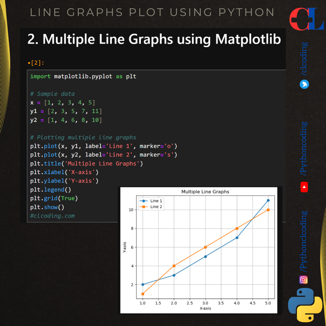
2. Multiple Line Graphs using Matplotlib

import matplotlib.pyplot as plt

# Sample data

x = [1, 2, 3, 4, 5]

y1 = [2, 3, 5, 7, 11]

y2 = [1, 4, 6, 8, 10]

# Plotting multiple line graphs

plt.plot(x, y1, label='Line 1', marker='o')

plt.plot(x, y2, label='Line 2', marker='s')

plt.title('Multiple Line Graphs')

plt.xlabel('X-axis')

plt.ylabel('Y-axis')

plt.legend()

plt.grid(True)

plt.show()

1. Basic Line Graph using Matplotlib

import matplotlib.pyplot as plt

# Sample data

x = [1, 2, 3, 4, 5]

y = [2, 3, 5, 7, 11]

# Plotting the line graph

plt.plot(x, y, marker='o')

plt.title('Basic Line Graph')

plt.xlabel('X-axis')

plt.ylabel('Y-axis')

plt.grid(True)

plt.show()

Read More

5 Practical Examples to Master Python Decorators

 

5. Decorator for Timing

A decorator to measure the execution time of a function.

import time

def timer(func):

    def wrapper(*args, **kwargs):

        start_time = time.time()

        result = func(*args, **kwargs)

        end_time = time.time()

        print(f"{func.__name__} executed in {end_time - start_time} seconds")

        return result

    return wrapper

@timer

def slow_function():

    time.sleep(2)

    return "Finished"

print(slow_function())

#clcoding.com

slow_function executed in 2.001049518585205 seconds

Finished

4. Decorator for Caching

A decorator to cache the results of expensive function calls.

def cache(func):

    cached_results = {}

    def wrapper(*args):

        if args in cached_results:

            return cached_results[args]

        result = func(*args)

        cached_results[args] = result

        return result

    return wrapper

@cache

def slow_function(x):

    print(f"Computing {x}...")

    return x * x

print(slow_function(4))

print(slow_function(4))

print(slow_function(5))

#clcoding.com

Computing 4...

16

16

Computing 5...

25

3. Decorator for Logging

A decorator to log function calls and their arguments.

def logger(func):

    def wrapper(*args, **kwargs):

        print(f"Function {func.__name__} called with args: {args} and kwargs: {kwargs}")

        result = func(*args, **kwargs)

        print(f"Function {func.__name__} returned {result}")

        return result

    return wrapper

@logger

def add(a, b):

    return a + b

add(3, 5)

#clcoding.com

Function add called with args: (3, 5) and kwargs: {}

Function add returned 8

8

2. Decorator with Arguments

A decorator that accepts arguments to customize its behavior.

def repeat(n):

    def decorator(func):

        def wrapper(*args, **kwargs):

            for _ in range(n):

                func(*args, **kwargs)

        return wrapper

    return decorator

@repeat(3)

def greet(name):

    print(f"Hello, {name}!")

greet("Clcoding")

#clcoding.com

Hello, Clcoding!

Hello, Clcoding!

Hello, Clcoding!

1. Basic Decorator

A simple example to understand the basic structure and functionality of decorators.

def simple_decorator(func):

    def wrapper():

        print("Before the function runs")

        func()

        print("After the function runs")

    return wrapper

@simple_decorator

def say_hello():

    print("Hello!")

say_hello()

#clcoding.com

Before the function runs

Hello!

After the function runs

Read More

Python Coding challenge - Day 233 | What is the output of the following Python Code?

 Let's break down the code and explain what each part does:

my_list = [1, 2, 3, 4, 5]

my_list[1:3] = []

print(my_list)

Step-by-Step Explanation

Create a List:

my_list = [1, 2, 3, 4, 5]

This line initializes a list named my_list with the elements [1, 2, 3, 4, 5].

Slice Assignment:

my_list[1:3] = []

my_list[1:3] is a slice of the list from index 1 to index 3, but not including index 3. In this case, my_list[1:3] refers to the sublist [2, 3].

The assignment my_list[1:3] = [] replaces the slice [2, 3] with an empty list [], effectively removing the elements 2 and 3 from the list.

Print the Modified List:

print(my_list)

This line prints the modified list.

After the slice assignment, my_list is modified to remove the elements at indices 1 and 2 (the elements 2 and 3). The resulting list is:

[1, 4, 5]

Visual Breakdown

Let's visualize the process:

Initial list: [1, 2, 3, 4, 5]

Slice my_list[1:3] refers to [2, 3]

Assigning [] to the slice removes [2, 3]

Resulting list: [1, 4, 5]

Full Code with Output

Here is the complete code along with its output:

my_list = [1, 2, 3, 4, 5]

my_list[1:3] = []

print(my_list)  # Output: [1, 4, 5]

The output is [1, 4, 5], as explained.

Read More

Function Interfaces in Python

 

10. Combining Concepts

def trace(func):

    

    """A decorator that traces function calls."""

    

    def wrapper(*args, **kwargs):

        print(f"TRACE: calling {func.__name__}() with {args}, {kwargs}")

        result = func(*args, **kwargs)

        print(f"TRACE: {func.__name__}() returned {result}")

        return result

    return wrapper

@trace

def compute_area(length: float, width: float) -> float:

    """Compute the area of a rectangle."""

    return length * width

area = compute_area(3.0, 4.5)

# clcoding.com

TRACE: calling compute_area() with (3.0, 4.5), {}

TRACE: compute_area() returned 13.5

9. Decorators

def debug(func):

    """A decorator that prints the function 

    signature and return value."""

    def wrapper(*args, **kwargs):

        print(f"Calling {func.__name__} with {args} and {kwargs}")

        result = func(*args, **kwargs)

        print(f"{func.__name__} returned {result}")

        return result

    return wrapper

@debug

def add(a, b):

    """Add two numbers."""

    return a + b

add(3, 4)

# clcoding.com

Calling add with (3, 4) and {}

add returned 7

7

8. Lambda Functions

square = lambda x: x * x

print(square(5))  

# clcoding.com

25

7. First-Class Functions

def square(x):

    """Return the square of x."""

    return x * x

def apply_function(func, value):

    """Apply a function to a value 

    and return the result."""

    return func(value)

result = apply_function(square, 4)

print(result)  

# clcoding.com

16

6. Docstrings

def divide(x, y):

    """

    Divide x by y and return the result.

    

    :param x: numerator

    :param y: denominator

    :return: division result

    """

    return x / y

result = divide(10, 2)

print(result)  

# clcoding.com

5.0

5. Function Annotations

def multiply(x: int, y: int) -> int:

    

    """Multiply two integers 

    and return the result."""

    

    return x * y

result = multiply(3, 4)

print(result)

# clcoding.com

12

4. Arbitrary Keyword Parameters

def print_info(**kwargs):

    

    """Print key-value pairs 

    from keyword arguments."""

    

    for key, value in kwargs.items():

        print(f"{key}: {value}")

print_info(name="Clcoding", age=30, city="Earth")

# clcoding.com

name: Clcoding

age: 30

city: Earth

3. Arbitrary Positional Parameters

def sum_all(*args):

    

    """Sum all given arguments."""

    

    return sum(args)

total = sum_all(1, 2, 3, 4, 5)

print(total)  

# clcoding.com

15

2. Keyword Parameters

def greet(name, greeting="Hello"):

    """Greet someone with a provided 

    greeting or a default greeting."""

    return f"{greeting}, {name}!"

message = greet("Clcoding")

print(message)  

message = greet("Python", "Hi")

print(message) 

# clcoding.com

Hello, Clcoding!

Hi, Python!

1. Basic Function Definition

def add(a, b):

    

    """Add two numbers and 

    return the result."""

    

    return a + b

result = add(3, 5)

print(result)  

# clcoding.com

8

Read More

10 Level of writing Python List

 Level 1: Basic List Creation

# Creating a simple list

my_list = [1, 2, 3, 4, 5]

print(my_list)

#clcoding.com

[1, 2, 3, 4, 5]

Level 2: Accessing List Elements

# Accessing elements by index

my_list = [1, 2, 3, 4, 5]

first_element = my_list[0]

last_element = my_list[-1]

print( "First:", first_element, "Last:", last_element)

#clcoding.com

First: 1 Last: 5

Level 3: List Slicing

# Slicing a list

my_list = [1, 2, 3, 4, 5]

sub_list = my_list[1:4]

print(sub_list)

#clcoding.com

[2, 3, 4]

Level 4: Adding Elements to a List

# Appending and extending a list

my_list = [1, 2, 3, 4, 5]

my_list.append(6)

my_list.extend([7, 8])

print(my_list)

#clcoding.com

[1, 2, 3, 4, 5, 6, 7, 8]

Level 5: Removing Elements from a List

# Removing elements

my_list = [1, 2, 3, 4, 5]

my_list.remove(2)  

popped_element = my_list.pop()  

print(my_list)

print(popped_element)

#clcoding.com

[1, 3, 4]

5

Level 6: List Comprehensions

# Using list comprehensions

my_list = [1, 2, 3, 4, 5]

squared_list = [x**2 for x in my_list]

print(squared_list)

#clcoding.com

[1, 4, 9, 16, 25]

Level 7: Nested Lists

# Creating and accessing nested lists

nested_list = [[1, 2, 3], [4, 5, 6], [7, 8, 9]]

element = nested_list[1][2]  

print(nested_list, element)

#clcoding.com

[[1, 2, 3], [4, 5, 6], [7, 8, 9]] 6

Level 8: Using List Functions and Methods

# Using built-in functions and methods

my_list = [1, 2, 3, 4, 5]

length = len(my_list)

sorted_list = sorted(my_list)

my_list.sort(reverse=True)

print(length, sorted_list, my_list)

#clcoding.com

5 [1, 2, 3, 4, 5] [5, 4, 3, 2, 1]

Level 9: List Iteration

# Iterating over a list

for element in my_list:

    print(element)

5

4

3

2

1

Level 10: Advanced List Operations

# Using advanced operations like map, filter, and reduce

my_list = [1, 2, 3, 4, 5]

from functools import reduce

# Map: applying a function to each element

doubled_list = list(map(lambda x: x * 2, my_list))

print(doubled_list)

# Filter: filtering elements based on a condition

even_list = list(filter(lambda x: x % 2 == 0, my_list))

print(even_list)

# Reduce: reducing the list to a single value

sum_of_elements = reduce(lambda x, y: x + y, my_list)

print(sum_of_elements)

#clcoding.com

[2, 4, 6, 8, 10]

[2, 4]

15

Read More

6 Things I Wish I Knew Earlier About Python Numbers

 

6. Fraction Module for Rational Numbers

The fractions module provides support for rational number arithmetic.

from fractions import Fraction

a = Fraction(1, 3)

b = Fraction(2, 3)

c = a + b

print(c)  

#clcoding.com

1

5. Decimal Module for Precise Calculations

For financial and other applications requiring precise decimal representation, the decimal module is very useful.

from decimal import Decimal, getcontext

getcontext().prec = 6  

a = Decimal('0.1')

b = Decimal('0.2')

c = a + b

print(c)  

#clcoding.com

0.3

4. Built-In Functions for Numerical Operations

Python provides several built-in functions to perform various numerical operations, such as abs(), round(), pow(), and many more.

print(abs(-5))  

print(round(3.14159, 2))  

print(pow(2, 3))  

#clcoding.com

5

3.14

8

3. Complex Numbers

Python natively supports complex numbers, which can be created by adding a 'j' or 'J' suffix to a number.

a = 3 + 4j  

print(a.real)  

print(a.imag)  

#clcoding.com

3.0

4.0

2. Floating-Point Precision

Floating-point numbers in Python are based on the IEEE 754 double-precision standard, which can lead to precision issues.

a = 0.1 + 0.2

print(a)  

#clcoding.com

0.30000000000000004

1. Integers Are of Arbitrary Precision

In Python, integers are of arbitrary precision, meaning they can grow as large as the memory allows. This is different from many other programming languages where integers have fixed sizes.

a = 10**100  

print(a)  

#clcoding.com

10000000000000000000000000000000000000000000000000000000000000000000000000000000000000000000000000000

Read More

Foundations of Data Structures and Algorithms Specialization

 

In the realm of computer science, data structures and algorithms are the backbone of efficient programming and software development. They form the fundamental concepts that every aspiring software engineer, data scientist, and computer scientist must master to solve complex problems effectively. Coursera's "Data Structures and Algorithms" Specialization, offered by the University of Colorado Boulder, provides an in-depth journey into these essential topics, equipping learners with the skills needed to excel in the tech industry.

Why Data Structures and Algorithms Matter

Data structures and algorithms are the building blocks of all software applications. They enable programmers to handle data efficiently, optimize performance, and ensure that applications run smoothly. Understanding these concepts is crucial for:

• Problem Solving: Algorithms provide a set of instructions to solve specific problems, while data structures organize and store data for efficient access and modification.
• Efficiency: Efficient algorithms and data structures improve the speed and performance of applications, making them scalable and robust.
• Competitive Programming: Mastery of these topics is essential for acing technical interviews and excelling in competitive programming contests.
• Software Development: From simple applications to complex systems, every software development project relies on the principles of data structures and algorithms.

Course Overview

The Coursera Specialization on Data Structures and Algorithms consists of several courses designed to take learners from basic to advanced levels. Here's a glimpse of what each course offers:

1. Algorithmic Toolbox:

   • Introduction to the basic concepts of algorithms.
   • Study of algorithmic techniques like greedy algorithms, dynamic programming, and divide-and-conquer.
   • Practical problem-solving sessions to reinforce learning.

2. Data Structures:

   • Comprehensive coverage of fundamental data structures such as arrays, linked lists, stacks, queues, trees, and graphs.
   • Exploration of advanced data structures like heaps, hash tables, and balanced trees.
   • Hands-on exercises to implement and manipulate various data structures.

3. Algorithms on Graphs:

   • Detailed study of graph algorithms including breadth-first search (BFS), depth-first search (DFS), shortest paths, and minimum spanning trees.
   • Real-world applications of graph algorithms in networking, web search, and social networks.

4. Algorithms on Strings:

   • Techniques for string manipulation and pattern matching.
   • Algorithms for substring search, text compression, and sequence alignment.
   • Applications in bioinformatics, data compression, and text processing.

5. Advanced Algorithms and Complexity:

   • Exploration of advanced topics such as NP-completeness, approximation algorithms, and randomized algorithms.
   • Analysis of algorithmic complexity and performance optimization.

Key Features

• Expert Instruction: The courses are taught by experienced professors from the University of Colorado Boulder, ensuring high-quality instruction and guidance.
• Interactive Learning: Each course includes a mix of video lectures, quizzes, programming assignments, and peer-reviewed projects to enhance learning.
• Flexibility: Learners can progress at their own pace, making it convenient to balance studies with other commitments.
• Certification: Upon completion, participants receive a certificate that can be shared on LinkedIn and added to their resumes, showcasing their proficiency in data structures and algorithms.

Who Should Enroll? Foundations of Data Structures and Algorithms Specialization

This specialization is ideal for:

• Aspiring Programmers: Beginners looking to build a strong foundation in data structures and algorithms.
• Software Engineers: Professionals seeking to improve their problem-solving skills and prepare for technical interviews.
• Computer Science Students: Individuals aiming to deepen their understanding of core computer science concepts.
• Tech Enthusiasts: Anyone with a passion for technology and a desire to learn how to solve complex problems efficiently.

Conclusion

Mastering data structures and algorithms is a crucial step towards becoming a proficient software engineer and problem solver. Coursera's "Data Structures and Algorithms" Specialization offers a comprehensive and structured learning path to achieve this mastery. With expert instruction, interactive learning experiences, and the flexibility to learn at your own pace, this specialization is an invaluable resource for anyone looking to excel in the tech industry.

Read More

Numerical Methods in Python

 

5. Runge-Kutta Method (RK4):

A fourth-order numerical method for solving ordinary differential equations (ODEs), more accurate than Euler's method for many types of problems.

def runge_kutta_4(func, initial_x, initial_y, step_size, num_steps):

    x = initial_x

    y = initial_y

    for _ in range(num_steps):

        k1 = step_size * func(x, y)

        k2 = step_size * func(x + step_size / 2, y + k1 / 2)

        k3 = step_size * func(x + step_size / 2, y + k2 / 2)

        k4 = step_size * func(x + step_size, y + k3)

        y += (k1 + 2*k2 + 2*k3 + k4) / 6

        x += step_size

    return x, y

# Example usage:

def dy_dx(x, y):

    return x + y

x_final, y_final = runge_kutta_4(dy_dx, initial_x=0, 

                                 initial_y=1, step_size=0.1, num_steps=100)

print(f"At x = {x_final}, y = {y_final}")

#clcoding.com

At x = 9.99999999999998, y = 44041.593801752446

4. Bisection Method:

A root-finding algorithm that repeatedly bisects an interval and then selects a subinterval in which a root must lie for further processing.

def bisection_method(func, a, b, tolerance=1e-10, max_iterations=100):

    if func(a) * func(b) >= 0:

        raise ValueError("Function does not change sign over interval")

    

    for _ in range(max_iterations):

        c = (a + b) / 2

        if abs(func(c)) < tolerance:

            return c

        if func(c) * func(a) < 0:

            b = c

        else:

            a = c

    raise ValueError("Failed to converge")

# Example usage:

def h(x):

    return x**3 - 2*x - 5

root = bisection_method(h, a=2, b=3)

print(f"Root found at x = {root}")

#clcoding.com

Root found at x = 2.0945514815393835

3. Secant Method:

A root-finding algorithm that uses a succession of roots of secant lines to better approximate a root of a function.

def secant_method(func, x0, x1, tolerance=1e-10, max_iterations=100):

    for _ in range(max_iterations):

        fx1 = func(x1)

        if abs(fx1) < tolerance:

            return x1

        fx0 = func(x0)

        denominator = (fx1 - fx0) / (x1 - x0)

        x_next = x1 - fx1 / denominator

        x0, x1 = x1, x_next

    raise ValueError("Failed to converge")

# Example usage:

def g(x):

    return x**3 - 2*x - 5

root = secant_method(g, x0=2, x1=3)

print(f"Root found at x = {root}")

#clcoding.com

Root found at x = 2.094551481542327

2. Euler's Method:

A first-order numerical procedure for solving ordinary differential equations (ODEs).

def euler_method(func, initial_x, initial_y, step_size, num_steps):

    x = initial_x

    y = initial_y

    for _ in range(num_steps):

        y += step_size * func(x, y)

        x += step_size

    return x, y

# Example usage:

def dy_dx(x, y):

    return x + y

x_final, y_final = euler_method(dy_dx, initial_x=0, 

                                initial_y=1, step_size=0.1, num_steps=100)

print(f"At x = {x_final}, y = {y_final}")

#clcoding.com

At x = 9.99999999999998, y = 27550.224679644543

1. Newton-Raphson Method:

Used for finding successively better approximations to the roots (or zeroes) of a real-valued function.

import numdifftools as nd

def newton_raphson(func, initial_guess, tolerance=1e-10, max_iterations=100):

    x0 = initial_guess

    for _ in range(max_iterations):

        fx0 = func(x0)

        if abs(fx0) < tolerance:

            return x0

        fprime_x0 = nd.Derivative(func)(x0)

        x0 = x0 - fx0 / fprime_x0

    raise ValueError("Failed to converge")

# Example usage:

import math

def f(x):

    return x**3 - 2*x - 5

root = newton_raphson(f, initial_guess=3)

print(f"Root found at x = {root}")

#clcoding.com

Root found at x = 2.0945514815423474

Read More

Top 3 Python Tools for Stunning Network Graphs

 

Top 3 Python Tools for Stunning Network Graphs

1. NetworkX

NetworkX is a powerful library for the creation, manipulation, and study of complex networks. It provides basic visualization capabilities, which can be extended using Matplotlib.

import networkx as nx

import matplotlib.pyplot as plt

# Create a graph

G = nx.erdos_renyi_graph(30, 0.05)

# Draw the graph

nx.draw(G, with_labels=True, node_color='skyblue', node_size=30, edge_color='gray')

plt.show()

No description has been provided for this image

2. Pyvis

Pyvis is a library built on top of NetworkX that allows for interactive network visualization in web browsers. It uses the Vis.js library to create dynamic and interactive graphs.

from pyvis.network import Network

import networkx as nx

# Create a graph

G = nx.erdos_renyi_graph(30, 0.05)

# Initialize Pyvis network

net = Network(notebook=True)

# Populate the network with nodes and edges from NetworkX graph

net.from_nx(G)

# Show the network

net.show("network.html")

#clcoding.com

Warning: When  cdn_resources is 'local' jupyter notebook has issues displaying graphics on chrome/safari. Use cdn_resources='in_line' or cdn_resources='remote' if you have issues viewing graphics in a notebook.

network.html

3. Plotly

Plotly is a graphing library that makes interactive, publication-quality graphs online. It supports interactive network graph visualization

import plotly.graph_objects as go

import networkx as nx

# Create a graph

G = nx.random_geometric_graph(200, 0.125)

# Extract the positions of nodes

pos = nx.get_node_attributes(G, 'pos')

# Create the edges

edge_x = []

edge_y = []

for edge in G.edges():

    x0, y0 = pos[edge[0]]

    x1, y1 = pos[edge[1]]

    edge_x.extend([x0, x1, None])

    edge_y.extend([y0, y1, None])

edge_trace = go.Scatter(

    x=edge_x, y=edge_y,

    line=dict(width=0.5, color='#888'),

    hoverinfo='none',

    mode='lines')

# Create the nodes

node_x = []

node_y = []

for node in G.nodes():

    x, y = pos[node]

    node_x.append(x)

    node_y.append(y)

node_trace = go.Scatter(

    x=node_x, y=node_y,

    mode='markers',

    hoverinfo='text',

    marker=dict(

        showscale=True,

        colorscale='YlGnBu',

        size=10,

        colorbar=dict(

            thickness=15,

            title='Node Connections',

            xanchor='left',

            titleside='right'

        )))

# Combine the traces

fig = go.Figure(data=[edge_trace, node_trace],

                layout=go.Layout(

                    title='Network graph made with Python',

                    showlegend=False,

                    hovermode='closest',

                    margin=dict(b=20, l=5, r=5, t=40),

                    xaxis=dict(showgrid=False, zeroline=False),

                    yaxis=dict(showgrid=False, zeroline=False)))

# Show the plot

fig.show()

 

Read More

Python Coding challenge - Day 232 | What is the output of the following Python Code?

 

Code:

class MyClass:

    def __init__(self, value):

        self.value = value

    def print_value(self):

        print(self.value)

obj = MyClass(30)

obj.print_value()

Solution and Explanantion: 

Let's break down the code step by step:

Class Definition

class MyClass:

This line defines a new class named MyClass. A class is a blueprint for creating objects, which are instances of the class.

Constructor Method

    def __init__(self, value):

        self.value = value

The __init__ method is a special method in Python known as the constructor. It is called when an object is created from the class and allows the class to initialize the attributes of the object.

self is a reference to the current instance of the class. It is used to access variables that belong to the class.

value is a parameter that is passed to the constructor when an object is created.

self.value = value assigns the passed value to the instance variable value.

Instance Method

    def print_value(self):

        print(self.value)

This is a method defined within the class. It takes self as an argument, which allows it to access the instance's attributes and methods.

print(self.value) prints the value of the value attribute of the instance.

Creating an Object

obj = MyClass(30)

Here, an instance of MyClass is created with the value 30. This calls the __init__ method, setting the instance's value attribute to 30.

Calling a Method

obj.print_value()

This line calls the print_value method on the obj instance, which prints the value of the instance's value attribute to the console. In this case, it will print 30.

Summary

The entire code does the following:

Defines a class MyClass with an __init__ method for initialization and a print_value method to print the value attribute.

Creates an instance of MyClass with a value of 30.

Calls the print_value method on the instance, which prints 30.

Read More

Screenshot in Python

 import pyautogui

from PIL import Image

# Take a screenshot

myScreenshot = pyautogui.screenshot()

# Save the screenshot

myScreenshot.save(r'ss_clcoding.png')

# Open the screenshot image

Image.open(r'ss_clcoding.png')

#clcoding.com

Read More

Python Coding challenge - Day 231 | What is the output of the following Python Code?

 

Code:

class MyClass:

    class_attribute = 10

    def __init__(self, value):

        self.instance_attribute = value

obj = MyClass(20)

print(obj.class_attribute)

Solution and Explanation: 

Let's break down the code step by step:

Class Definition

class MyClass:

This line defines a new class named MyClass. A class is a blueprint for creating objects (instances).

Class Attribute

    class_attribute = 10

Within the class definition, class_attribute is defined. This is a class attribute, which means it is shared by all instances of the class. You can access this attribute using the class name (MyClass.class_attribute) or any instance of the class (obj.class_attribute).

Constructor Method

    def __init__(self, value):

        self.instance_attribute = value

This is the constructor method (__init__). It is called when an instance of the class is created. The self parameter refers to the instance being created. The value parameter is passed when creating an instance. Inside the method, self.instance_attribute = value sets an instance attribute named instance_attribute to the value passed to the constructor.

Creating an Instance

obj = MyClass(20)

Here, an instance of MyClass is created, and the value 20 is passed to the constructor. This means obj.instance_attribute will be set to 20.

Accessing the Class Attribute

print(obj.class_attribute)

This line prints the value of class_attribute using the instance obj. Since class_attribute is a class attribute, its value is 10.

Summary

class_attribute is a class attribute shared by all instances of MyClass.

instance_attribute is an instance attribute specific to each instance.

obj = MyClass(20) creates an instance with instance_attribute set to 20.

print(obj.class_attribute) prints 10, the value of the class attribute.

So, the output of the code will be:

10

Read More

Asynchronous Programming in Python

 

Asynchronous programming in Python is a powerful technique for improving the performance of programs that involve I/O-bound tasks such as network requests, file operations, and database interactions. By allowing for concurrent execution of code, asynchronous programming can make your applications faster and more efficient. In this blog, we will delve into the key concepts, components, and practical examples of asynchronous programming in Python.

Understanding the Basics

1. Event Loop The event loop is the core of asynchronous programming. It continuously runs, checking for and executing tasks, including I/O operations and user-defined coroutines. It manages when and what to execute, enabling concurrent execution.

2. Coroutine A coroutine is a special type of function declared with async def and run with await. Coroutines can pause and resume their execution, allowing other tasks to run concurrently. This is the cornerstone of writing asynchronous code in Python.

3. await Keyword The await keyword is used to pause the execution of a coroutine until the awaited task is completed. It must be used within an async def function. This mechanism allows other tasks to run while waiting for the result of the awaited task.

4. asyncio Library asyncio is the primary library for asynchronous programming in Python. It provides the event loop, coroutine management, and various utilities for asynchronous I/O operations.

Example of Asynchronous Programming

Let's look at a simple example of asynchronous programming using the asyncio library:

import asyncio

async def fetch_data():

    print("Start fetching data")

    await asyncio.sleep(2)  # Simulate an I/O operation with asyncio.sleep

    print("Data fetched")

    return {"data": "sample"}

async def main():

    print("Start main")

    data = await fetch_data()  # Await the coroutine fetch_data

    print("Received data:", data)

    print("End main")

# Run the main coroutine

asyncio.run(main())

In this example, the fetch_data coroutine simulates an I/O operation using await asyncio.sleep(2), pausing its execution for 2 seconds. The main coroutine awaits the fetch_data coroutine, allowing it to run concurrently with other tasks if there were any.

Key Functions and Classes in asyncio

• asyncio.run(coroutine): Runs the main coroutine and manages the event loop.
• asyncio.create_task(coroutine): Schedules a coroutine to run concurrently as a Task.
• await asyncio.sleep(seconds): Suspends the coroutine for the specified number of seconds, useful for simulating I/O operations.

Advanced Features

Asynchronous Generators Asynchronous generators are declared with async def and use yield to produce values. They are useful for creating asynchronous iterables, allowing you to work with streams of data asynchronously.

Asynchronous Context Managers Asynchronous context managers, declared with async with, ensure proper resource management in asynchronous code. They are particularly useful for handling resources like file handles or network connections that need to be cleaned up after use.

Using Third-Party Libraries

To extend the capabilities of asyncio, you can use third-party libraries like aiohttp for asynchronous HTTP requests and aiomysql for asynchronous database interactions. Here’s an example using aiohttp:

import aiohttp

import asyncio

async def fetch_page(url):

    async with aiohttp.ClientSession() as session:

        async with session.get(url) as response:

            return await response.text()

async def main():

    url = "https://example.com"

    html = await fetch_page(url)

    print(html)

# Run the main coroutine

asyncio.run(main())

In this example, aiohttp is used to perform an asynchronous HTTP GET request. The fetch_page coroutine makes the request and awaits the response, allowing other tasks to run concurrently.

Conclusion

Asynchronous programming in Python is a powerful way to handle tasks concurrently, making programs more efficient, especially for I/O-bound operations. By understanding and utilizing the event loop, coroutines, and the asyncio library, you can significantly improve the performance of your Python applications. Additionally, leveraging advanced features and third-party libraries like aiohttp can further extend the capabilities of your asynchronous code. Embrace the power of asynchronous programming and unlock the full potential of Python in your projects!

Read More